


ARIMA ETS TBATS forecasting models are the three workhorses of traditional time-series analysis — yet most businesses apply them without understanding which one actually fits their data. After testing all three on four years of identical sales data, the results surprised everyone in the room. The simplest model delivered the highest accuracy. The most sophisticated algorithm performed worst.
Comparing ARIMA ETS and TBATS forecasting models reveals an uncomfortable truth: complexity doesn’t guarantee accuracy. The best model for your business depends on your specific data patterns, not which algorithm sounds most impressive in presentations.
This article dissects all three ARIMA ETS TBATS forecasting methods, showing you exactly when each one excels and when it fails. You’ll see real accuracy metrics from identical test data, learn how to interpret model outputs, and walk away with a practical decision framework.
If you’re new to forecasting concepts, start with our introduction to sales forecasting that covers data preparation and fundamental principles.
Table of Contents
How ARIMA Forecasting Works
Think of ARIMA as a sophisticated pattern recognition system built from three interlocking mechanisms:
Auto-Regressive (AR): Today’s sales correlate with recent history. If you sold $95K last month and $98K the month before, next month probably lands in that range rather than suddenly jumping to $150K.
Integrated (I): Removes trends by differencing. If sales grow 3% monthly, ARIMA strips out that consistent growth to focus on the pattern underneath. This “stationarity” transformation lets the model see seasonal fluctuations more clearly.
Moving Average (MA): Learns from past prediction errors. If the model consistently underestimates December sales by $12K, it adjusts future December predictions upward.
When ARIMA Excels and When It Struggles
ARIMA performs best when your data shows:
- Consistent patterns: Seasonal cycles that repeat predictably year-over-year
- Linear trends: Steady growth or decline without sudden jumps
- Stable structure: No major business changes during the historical period
- Sufficient history: At least 3 years (36 months) of clean data
ARIMA struggles with:
- Structural breaks: Acquisitions, new product launches, market disruptions
- Multiple seasonality: Weekly AND monthly AND yearly patterns simultaneously
- Irregular holidays: Easter, Ramadan, Chinese New Year (dates shift annually)
For most retail, manufacturing, and subscription businesses with stable operations, ARIMA delivers excellent results with minimal tuning required.
ETS Forecasting: The Exponential Smoothing Model
ETS forecasting (Error, Trend, Seasonality) takes a fundamentally different approach than ARIMA. Instead of analyzing correlations between time periods, it decomposes your data into three components and forecasts each separately.
How ETS Works
The ETS framework explicitly models three elements:
Error (E): Can be additive (constant variance) or multiplicative (variance grows with level)
Trend (T): None, additive (linear), or damped (growth slows over time)
Seasonality (S): None, additive (constant seasonal effect), or multiplicative (seasonal effect grows)
When ETS Excels and When It Struggles
ETS shines in specific scenarios:
- Strong recent patterns: When last quarter matters more than two years ago
- Proportional seasonality: Holiday sales grow with business size
- Interpretability priority: Business stakeholders understand “trend + seasonal effect”
- Forecasting speed: Computationally faster than ARIMA for large datasets
ETS struggles with:
- Complex autocorrelation: Patterns ARIMA captures through AR/MA terms
- Non-seasonal trends: ARIMA’s differencing handles these more flexibly
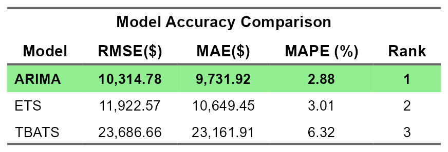
The performance gap (8.47% vs 2.88% MAPE) suggests this dataset has autocorrelation patterns that ARIMA captures but ETS misses.
TBATS Forecasting: Handling Complex Seasonality
TBATS forecasting represents the most sophisticated of the three traditional models, designed specifically for complex seasonality situations. The acronym describes its five components:
Trigonometric seasonality representation (using Fourier terms)
Box-Cox transformation (handles non-constant variance)
ARMA errors (captures autocorrelation)
Trend component
Seasonal components (multiple if needed)
How TBATS Works
Unlike ARIMA and ETS which assume single seasonality (monthly or quarterly), TBATS handles multiple overlapping seasonal patterns. Think of a hotel with:
- Weekly patterns (weekends vs weekdays)
- Monthly patterns (month-end business travel)
- Yearly patterns (summer vacation season)
TBATS uses trigonometric functions to represent these cycles simultaneously without requiring massive parameter counts.
When TBATS Excels and When It Struggles
TBATS justifies its complexity when you have:
- Multiple seasonality: Daily + weekly + yearly patterns
- Non-integer seasonality: 365.25 days/year, 52.18 weeks/year
- Calendar effects: Ramadan, Easter, Chinese New Year (floating dates)
- High-frequency data: Hourly utility usage, daily website traffic
TBATS struggles with:
- Simple patterns: Overkill that introduces unnecessary complexity
- Limited data: Needs substantial history to estimate many parameters
- Computational cost: Significantly slower than ARIMA/ETS
For monthly business data with straightforward yearly seasonality, TBATS adds complexity without accuracy gains — as the results below demonstrate.
ARIMA vs ETS vs TBATS: Head-to-Head Accuracy Comparison
Testing all three ARIMA ETS TBATS forecasting models on identical data reveals clear winners and losers:
ARIMA dominates across all metrics. TBATS performs around 6.3% MAPE — roughly 2× worse than ARIMA.
Why ARIMA Won This ARIMA ETS TBATS Forecasting Test
This dataset exhibits four characteristics that favour ARIMA over ETS and TBATS:
- Strong autocorrelation: Current sales correlate tightly with recent history
- Clean seasonality: Predictable yearly patterns without multiple overlapping cycles
- Stable structure: No major business disruptions during the 4-year period
- Sufficient data: 60 months provides adequate training observations
The data sits squarely in ARIMA’s sweet spot — TBATS’s complexity is not needed here.
Interpreting Confidence Intervals in Forecasting Models
All three ARIMA ETS TBATS forecasting models generate confidence intervals alongside point forecasts. Understanding these ranges matters more than the single prediction number.
The 80% vs 95% Interval Explained
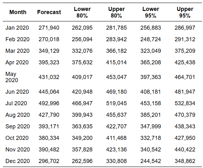
80% confidence interval [$262,095 – $281,785]: There is an 80% probability actual sales fall within this range. Conversely, 20% of the time reality falls outside these bounds.
95% confidence interval [$256,883 – $286,997]: Higher confidence requires wider bounds. You’re 95% certain actual sales land here, but the range spans $30,114.
Using Intervals for Business Decisions
Conservative inventory planning might use the upper 80% bound ($281,785) to ensure you rarely stock out. You’ll occasionally have excess, but customer satisfaction stays high.
Cash flow planning might use the lower 80% bound ($262,095) to ensure you can cover commitments even in below-forecast scenarios.
The point forecast ($271,940) represents the most likely outcome, but planning solely to that number ignores inherent uncertainty. Learn more about uncertainty quantification in business planning from Harvard Business Review.
Decision Framework: Which ARIMA ETS TBATS Forecasting Model Should You Use?
Follow this hierarchy when choosing between ARIMA ETS TBATS forecasting models for your business data:
Start with ARIMA if:
✅ You have 36+ months of historical data
✅ Patterns are relatively consistent year-over-year
✅ You need maximum accuracy
✅ You can explain “autocorrelation” to stakeholders (or they don’t ask)
Switch to ETS if:
✅ ARIMA accuracy disappoints
✅ You need faster computation (large product catalogs)
✅ Business users want interpretable components (trend + seasonal)
✅ Recent patterns matter more than distant history
Choose TBATS only if:
✅ You have multiple overlapping seasonal patterns
✅ Data frequency is high (daily/hourly)
✅ Standard models fail to capture complexity
✅ Computational time isn’t a constraint
Practical Implementation: Model Refresh Frequency
Whichever of the ARIMA ETS TBATS forecasting methods you select, keeping models current is essential. How often should you retrain with new data?
Monthly refresh: Appropriate for stable businesses where patterns change slowly. Retrain the first week of each month with the newly completed month’s data.
Quarterly refresh: Sufficient for businesses with low volatility and strong seasonal patterns that don’t shift.
Event-driven refresh: Retrain immediately after major changes — new product launch, competitive threat, or market disruption. Any structural break will degrade all three model types until they’re retrained on post-event data.
What’s Next: Machine Learning Forecasting Methods
Traditional ARIMA ETS TBATS forecasting models form the foundation of professional time-series analysis. They’re fast, interpretable, and often sufficient. But modern approaches offer compelling advantages in specific scenarios.
The next article explores machine learning sales forecasting with XGBoost — an optimised gradient boosting algorithm for classification and regression tasks.
Continue to Article 3: Machine Learning Method for Business Forecasting →